
Sizing a static mixer is not a black art — it is a six-decision procedure. You collect the process data, define the mixture quality target, select the geometry, fix the diameter, set the element count, and verify the pressure-drop budget. Work through them in order and the result is a mixer that meets the CoV target at the lowest lifetime cost. Skip one, and the failure modes are predictable: a mixer that under-mixes at turndown, or one that starves the pump at peak flow.
Step 1: Collect the Process Data
Start with the flow rates of every stream — at design conditions and at turndown, because a mixer sized only for design flow can sit far outside its operating window during startup or low-season operation. Record density and viscosity for each component and for the expected mixture, plus the full operating temperature range: viscosity can swing by a factor of three between a summer design case and a winter startup, and the pressure drop follows it. Finally, note the line size, the pipe material, and the pressure budget the pump can actually spare.
This mirrors the specification checklist used across the industry — Statiflo's static mixer design guide, for example, asks for component flow rates, densities, viscosities, design temperature and pressure, materials of construction, preferred pipe diameter, and the maximum permissible pressure drop before any geometry is proposed. One detail matters more than newcomers expect: the viscosity ratio between the streams. Dosing 0.1% of an additive into a clean main stream and blending two streams 50/50 at the same total flow are different sizing problems.
Step 2: Define the Mixture Quality Target
Mixture quality is expressed as σX (sigma-X) — the relative standard deviation of concentration measured across the outlet cross-section, often called the coefficient of variation (CoV). As a rule of thumb from published mixer specifications: additive dosing duty is typically targeted at σX ≤ 5%; continuous process blending sits in the 1-5% band depending on L/D and element count; and reaction duty where local concentration gradients affect selectivity justifies the tighter end of that band. Do not over-specify. In the laminar regime the pressure drop scales roughly with the square of the element count, so demanding a 1% uniformity where 5% would do can quadruple the pumping penalty for nothing.
Step 3: Select the Geometry by Viscosity and Flow Regime
Compute the pipe Reynolds number at the design flow. The regime decides which geometry is in its element, and the published specification ranges for our three core models bracket nearly every duty:
| Model | Viscosity Range | Dispersion Precision | σX Target | Typical Elements |
|---|---|---|---|---|
| SV corrugated plate | ≤ 100 cP | 1-2 μm (turbulent) / 3-5 μm (laminar) | ≤ 1-5% | 4-6 (turbulent) / 6-10 (laminar) |
| SX cross-bar | 1 - 10,000 cP | 2-5 μm | ≤ 1-5% (4-6 el.; 6-10 transitional Re) | 4-10 |
| SK helical | 1 cP - 10⁶ cP | ≤ 10 μm | ≤ 5% (5-8 el. at 180° / 4-6 el. at 270°) | 4-8 |
A useful sanity check on the regime question comes from Becht Engineering's inline mixing guide: at a Reynolds number of 100,000 or more, roughly 100 pipe diameters of empty pipe will blend two streams to about 95% mixedness. That is why long transfer lines sometimes "get away" with no mixer at all in hard-turbulent service — and why a static mixer earns its keep by delivering better uniformity in about 1% of that length, and by working at all in the transitional and laminar regimes where eddy diffusion is gone and the elements must do the stretching and folding themselves.
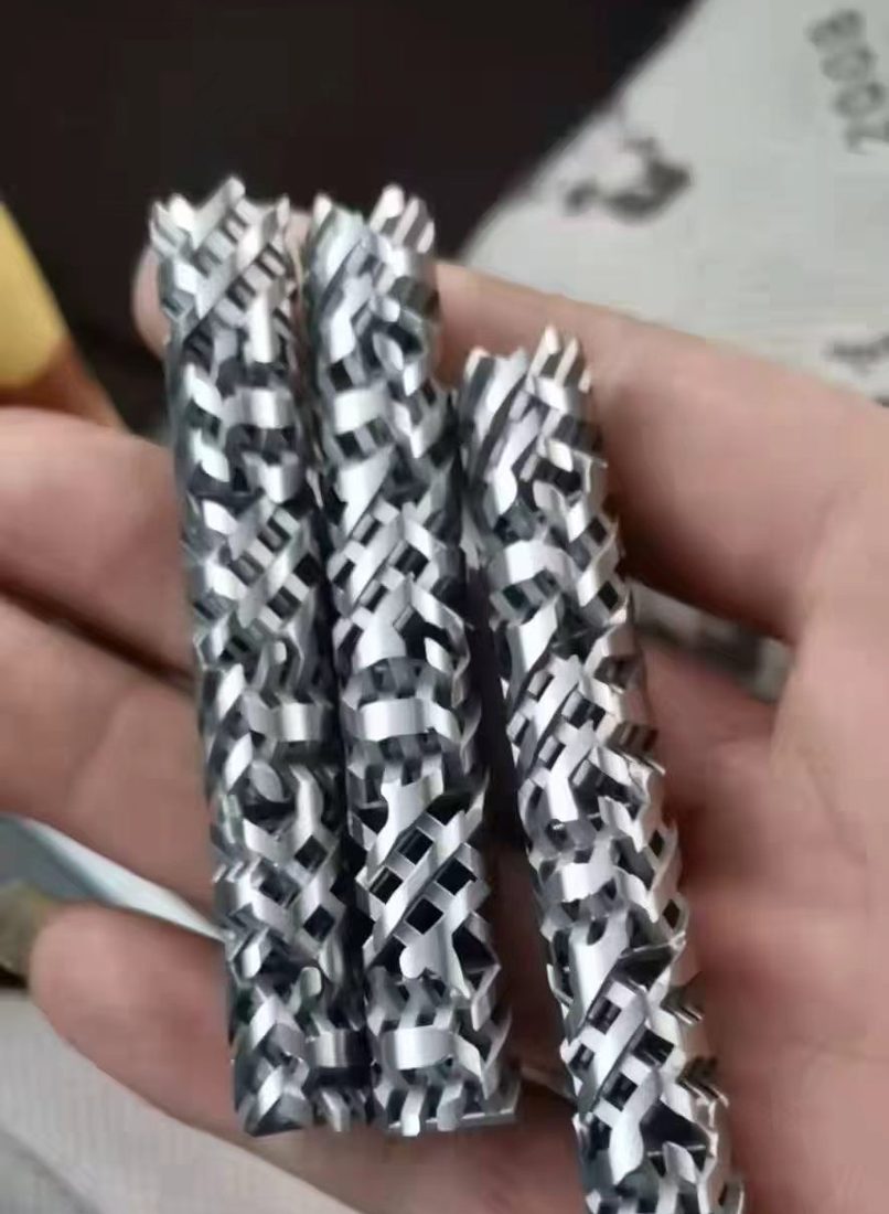
Step 4: Fix the Diameter from the Velocity Window
For low-viscosity liquids, aim for a superficial velocity of 1-2 m/s; for viscous media, 0.1-0.5 m/s. The lower bound matters as much as the upper one: below roughly 0.3 m/s the flow regime can transition to laminar and the mixing performance degrades exactly when the process is at turndown. The diameter falls out of the flow rate once the velocity window is chosen — DN50 carries about 12 m³/h at 1.5 m/s, DN80 about 26 m³/h, and DN100 about 45 m³/h. If the existing line is one or two sizes off the window, weigh the cost of a reducer set against the pressure-drop consequences of living with the wrong velocity for the whole life of the installation.
Step 5: Set the Element Count and Check the Pressure-Drop Budget
With geometry and diameter fixed, the element count is the knob that reaches the σX target from Step 2 — use the model-specific counts in the table above, and the calculation methods in our pressure drop calculation guide to verify the penalty. Compare the result against the application budget: low-pressure dosing loops tolerate 0.05-0.1 bar, standard process lines with a centrifugal pump typically carry a 0.2-0.5 bar budget, and viscous blending duty runs 1-3 bar. Always check the budget at peak flow, not just design flow: at 130% of design, the turbulent pressure drop is about 1.69 times the design value.
Worked example — dosing duty in DN80. River water, 25 m³/h, with a ferric coagulant side-dose. At DN80 (inner diameter 81 mm) the velocity is 1.35 m/s — inside the window — and the Reynolds number is about 109,000, hard-turbulent. The fluid is water-like, so the SV geometry fits (≤ 100 cP) with fine dispersion for the coagulant. Target σX ≤ 5%: six elements. Pressure drop by the empty-pipe method: friction factor f = 0.018 at this Reynolds number, mixer length L = 6 × 1.5 × D = 0.73 m, giving ΔP_pipe ≈ 144 Pa; with the SV geometry factor K = 5.5, the mixer drop is ≈ 790 Pa — about 0.008 bar, far inside any dosing budget. Residence time is 0.54 s. At 30% turndown the velocity is 0.40 m/s and the Reynolds number is still ≈ 33,000, so the mixing regime — and the spec — holds across the whole operating window.
Step 6: Close Out the Mechanical Details
Match the housing material to the service: our models are offered in SS304, SS316L, carbon steel, PVC, PP, and Hastelloy C-276. Connections are available as flanges (ANSI/DIN/JIS), threaded (NPT/BSP), welded, or Tri-Clamp for hygienic duty. In fouling or slurry service, specify removable elements so the stack can be inspected and cleaned through the flanges. Finally, write the σX target, the design flow window, and the calculated pressure drop into the datasheet — so that when the process debottleneck arrives two years later, the next engineer starts from facts instead of guesses.
Frequently Asked Questions
Component flow rates at design and turndown, density and viscosity of each stream, the operating temperature range, the pipe diameter and material, the allowable pressure drop, and the target mixture quality (σX). This is the same input set industry specification checklists — such as Statiflo's — request before proposing a geometry.
For additive dosing, σX ≤ 5% is the usual target. For continuous blending, published mixer specifications quote σX ≤ 1-5% depending on L/D and element count. Tighter targets cost elements, and in laminar flow each doubling of the element count roughly quadruples the pressure drop — so target what the process actually needs.
Most turbulent duties settle at 4-6 elements; laminar duties typically need 6-10. Model-specific figures: the SK helical mixer reaches σX ≤ 5% with 5-8 elements (180° twist) or 4-6 elements (270° twist), and the SX cross-bar mixer reaches σX ≤ 1-5% with 4-6 elements, or 6-10 in the transitional Reynolds band.
Verify both ends of the range. At 130% of design flow the turbulent pressure drop is about 1.69× the design value, so confirm the pump margin at peak. For a large planned increase, upsizing the diameter protects the pressure budget — but keep the minimum velocity above roughly 0.3-0.5 m/s so the flow regime, and with it the mixing performance, survives turndown.
That is the whole procedure: data, target, geometry, diameter, elements, budget. Send us your flow rate, viscosity, and pipe size and we will return a sized selection with the calculated σX and pressure drop within 24 hours.